Post-processing¶

Overview¶

RSKtools is RBR’s open source MATLAB toolbox for reading, post-processing, visualizing, and exporting RBR logger data. Users may plot data as a time series or as depth profiles using tailored plotting utilities. Time-depth heat maps can be plotted easily to visualise transects or moored profiler data. A full suite of data post-processing functionality, such as functions to match sensor time constants and bin average, are available to enhance data quality.

You may review the getting started guide for an introduction on how to open an RSK file and access data.

RSKtools includes a series of functions to post-process RBR logger data. Below we show how to implement some common processing steps to obtain the highest quality data possible. All post-processing functions are customisable via name-value pair input arguments. Documentation for each function can be accessed in MATLAB using help.

Note on multi-schedule RSK files¶

Unlike derive functions, post-processing functions are schedule-specific. Their default behaviour is to work on the auto-detected default schedule ('schedule', 'default'), which selects the schedule with the most Conductivity data, then Temperature, then schedule 1. If your RSK has multiple schedules, you can specify a schedule label explicitly (e.g., 'schedule', 's.CTD'). See the getting started guide for more information on multi-schedule support.

Basic Usage¶

rsk = RSKopen('sample.rsk');

% Print a list of all the channels in the RSK file
RSKprintchannels(rsk);

% Read profiles from the RSK file
rsk = RSKreadprofiles(rsk);

% Derive sea pressure from total pressure
rsk = RSKderiveseapressure(rsk);

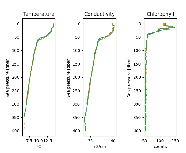
% Plot a few downcasts of temperature, conductivity, and chlorophyll
RSKplotprofiles(rsk, 'channel', {'Conductivity', 'Temperature', 'Chlorophyll'}, ...
                'profile', [1 2 3], 'direction', 'down');

Model:           RBRconcerto
Serial ID:       80231
Sampling period: 0.167 second
    index        channel             unit
    _____    ________________    _____________
    1        Conductivity        mS/cm
    2        Temperature         °C
    3        Pressure            dbar
    4        Dissolved O2        %
    5        Turbidity           NTU
    6        PAR                 µMol/m²/s
    7        Chlorophyll         µg/l

Derive sea pressure from total pressure¶

We suggest deriving sea pressure first, especially when an atmospheric pressure other than the nominal value of 10.1325 dbar is desired. The patm argument is the atmospheric pressure used to calculate the sea pressure. A custom value can be used; otherwise, the default is to retrieve the value stored in the parameters field or to assume it is 10.1325 dbar if the parameter’s field is unavailable. In this example, we take atmospheric pressure to be 10 dbar:

rsk = RSKderiveseapressure(rsk, 'patm', 10);

Data post-processing¶

What follows is a generic recipe for post-processing RBR CTD data. It is a guideline – RBR CTDs are used in many environments, with many sensor packages, and are profiled from a variety of vessels (or no vessel at all). While the basic approach here is relevant for many cases, the processing parameters may not apply widely.

First, keep a copy of the raw data to compare with the processed data later.

raw = rsk;

Correct for A2D zero-order hold¶

The analogue-to-digital (A2D) converter on RBR instruments must recalibrate periodically. In the time it takes for the calibration to finish, one or more samples are missed. The instrument firmware fills the missed sample with the same data measured during the previous sample, a technique called a zero-order hold. RSKcorrecthold() identifies zero-hold points by finding where consecutive differences of each channel are equal to zero and then replaces these samples with a NaN or an interpolated value.

rsk = RSKcorrecthold(rsk, 'action', 'interp');

Low-pass filtering¶

Low-pass filtering is commonly used to reduce noise and to match sensor time constants, typically for temperature and conductivity. Users may also wish to filter other channels to simply reduce noise (e.g., optical channels such as chlorophyll-a or turbidity).

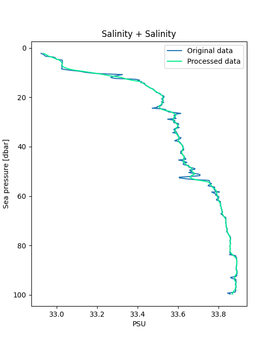
Most RBR instruments designed for profiling are equipped with thermistors that have a time constant of 100 ms, which is “slower” than the conductivity cell. When the time constants are different, salinity will contain spikes at strong gradients. One solution is to “slow down” the conductivity sensor to match the thermistor. In this example dataset, the logger sampled at 6 Hz, so a 5-sample running average provides more than sufficient smoothing to match the time response of the conductivity sensor to the thermistor.

rsk = RSKsmooth(rsk, 'channel', 'Salinity', 'windowLength', 5);

Alignment of conductivity and temperature¶

Conductivity and temperature often need to be aligned in time to account for the fact these sensors are not always co-located on the logger. The implication is that, under dynamic conditions (e.g., profiling), the sensors are measuring a slightly different parcel of water at any instant.

Furthermore, sensors with long time constants introduce a time lag to the data. For example, dissolved oxygen sensors often have a long time constant, and this delays the measurement relative to the true value. This can be fixed to some degree by advancing the sensor data in time.

When temperature and conductivity are misaligned, salinity will contain spikes at sharp interfaces and a bias in continuously stratified environments. Properly aligning the sensors, together with matching the time response, will minimise salinity spiking and bias.

A common approach to determine the optimal lag is to compute and plot salinity for a range of lags and choose the lag (often by eye) with the smallest salinity spikes at sharp temperature interfaces. RSKtools includes RSKcalculateCTlag() that estimates the optimal lag between conductivity and temperature by minimizing salinity spiking. We currently suggest using both approaches to check for consistency.

As a rough guide, temperature from a CTD equipped with the red combined CT cell and a fast thermistor typically requires only a very small-time advance (perhaps tens of milliseconds). Temperature from a CTD equipped with a cylindrical black conductivity cell (with the thermistor on the sensor endcap) typically requires a temperature lag correction of about 0.1 s to 0.3 s (1 or 2 samples at 6 Hz).

% Required shift of C relative to T for each profile
lag = RSKcalculateCTlag(rsk, 'seapressureRange', [1 50], 'direction', 'down');
% Advance temperature by the median lag
lag = -median(lag);
rsk = RSKalignchannel(rsk, 'channel', 'Temperature', 'lag', lag, 'direction', 'down');

Users wishing to learn more about dynamic sensor corrections and RBR CTDs are encouraged to watch a special RBR webinar on dynamic errors from May 2020 (Youtube and PDF).

Remove loops¶

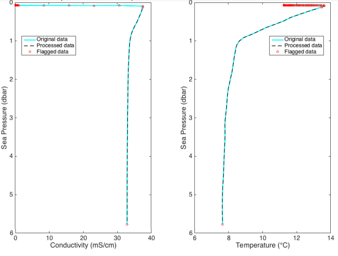
Working in rough seas can cause the CTD profiling rate to vary, and even change signs (i.e., the CTD momentarily changes direction). When this happens, the CTD effectively samples its own wake, degrading the quality of the profile in regions of strong gradients. The measurements taken when the instrument is profiling too slowly or during a pressure reversal should not be used for further analysis. We recommend using RSKremoveloops() to flag and treat the data when the instrument (1) falls below a threshold speed and (2) when the pressure reverses (the CTD “loops”). Before using RSKremoveloops(), use RSKderiveseapressure() to calculate sea pressure from total pressure, RSKderivedepth() to calculate depth from sea pressure, and then use RSKderivevelocity() to calculate profiling rate.

rsk = RSKderiveseapressure(rsk);
rsk = RSKderivedepth(rsk);
rsk = RSKderivevelocity(rsk);
% Apply the algorithm
rsk = RSKremoveloops(rsk, 'threshold', 0.3);

Derived variables¶

RSKtools includes a few convenience functions to derive common oceanographic variables. For example, RSKderivesalinity() computes Practical Salinity using the TEOS-10 GSW function gsw_SP_from_C, and adds a new channel called Salinity to the data. The TEOS-10 GSW MATLAB toolbox must be installed separately.

rsk = RSKderiveseapressure(rsk);
rsk = RSKderivedepth(rsk);
rsk = RSKderivevelocity(rsk);
rsk = RSKderivesalinity(rsk);
rsk = RSKderivesigma(rsk);

% Print a list of channels
RSKprintchannels(rsk);

Model:           RBRconcerto
Serial ID:       80231
Sampling period: 0.167 second
    index          channel              unit
    _____    ___________________    _____________
      Conductivity           mS/cm
      Temperature            °C
      Pressure               dbar
      Dissolved O2           %
      Turbidity              NTU
      PAR                    µMol/m²/s
      Chlorophyll            µg/l
      Sea Pressure           dbar
      Salinity               PSU
     Depth                  m
     Velocity               m/s
     Density Anomaly        kg/m³

Bin average all channels by sea pressure¶

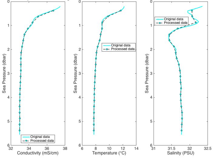
Bin averaging reduces sensor noise and ensures that each profile is referenced to a common grid. The latter is often an advantage for plotting data as “heatmaps.” RSKbinaverage() allows users to bin channels according to any reference, but the most common choices are time, depth, and sea pressure. It also can handle grids with a variable bin size. In the following example, the data are averaged into 0.25 dbar bins.

rsk = RSKbinaverage(rsk, 'binBy', 'Sea Pressure', 'binSize', 0.25, ...
                    'boundary', [0.5 5.5], 'direction', 'up');

Compare the raw and processed data¶

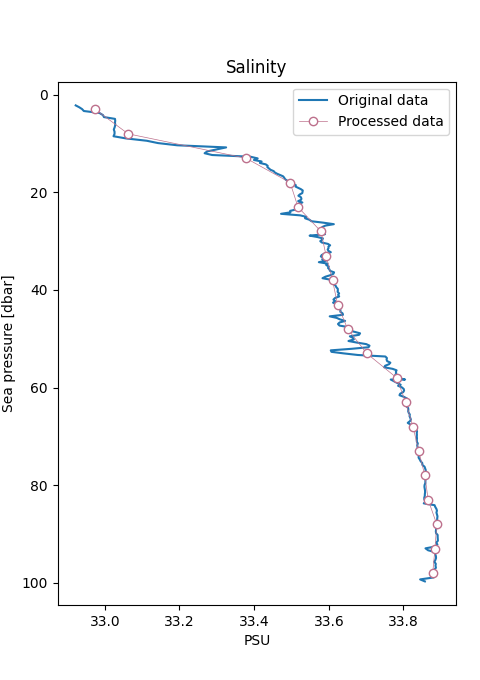
Use RSKplotprofiles() to compare the binned data to the raw data for a few example profiles.

figure;
RSKplotprofiles(raw, 'channel', {'Salinity'}, 'profile', 1, 'direction', 'down');
hold on;
RSKplotprofiles(rsk, 'channel', {'Salinity'}, 'profile', 1, 'direction', 'down');
hold off;

Visualise data with a 2D plot¶

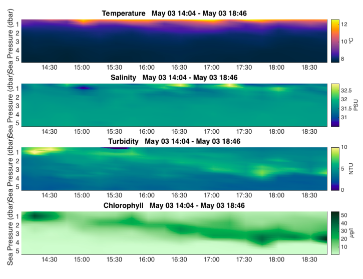
RSKimages() generates a time/depth heat-map of a channel. The x-axis is time; the y-axis is a reference channel (default is sea pressure). All the profiles must be evaluated on the same reference channel grid, which is accomplished with RSKbinaverage(). For more details, see RSKbinaverage() and RSKgenerate2D().

RSKimages(rsk, 'channel', {'Temperature', 'Salinity'}, 'direction', 'up');

Export logger data to CSV files¶

RSK2CSV() writes logger data and metadata to one or more CSV files. The CSV files contain a header with important logger metadata and a record of the processing steps made by RSKtools. The data table starts with a row of variable names and units above each column of channel data. If the profile number is specified, then one file will be written for each profile. Furthermore, an extra column called cast_direction will be included. Users can select which channels and profiles to write, the output directory, and also specify additional comments to be placed after the metadata in the file header.

RSK2CSV(rsk, 'channel', {'Depth', 'Temperature', 'Salinity'}, ...
        'profile', [1 2 3], 'comment', 'Processed with RSKtools');

RSKtools also has an export function to write Ruskin RSK files (see RSK2RSK()).

Display a summary of all the processing steps¶

disp(rsk.log);

Other Resources¶

We recommend reading the:

RSKtools API reference for detailed function documentation.
RSKtools getting started guide for an introduction on how to open an RSK file, make plots, and access the data.

About this document¶

The full source code for this documentation is located in the docs directory of the repository. All documentation is built and generated using Sphinx with the sphinxcontrib-matlabdomain extension.

RSKtools

Navigation

Related Topics