Getting started
Overview
RSKtools is RBR’s open source MATLAB toolbox for reading, post-processing, visualizing, and exporting RBR logger data. Users may plot data as a time series or as depth profiles using tailored plotting utilities. Time-depth heat maps can be plotted easily to visualise transects or moored profiler data. A full suite of data post-processing functionality, such as functions to match sensor time constants and bin average, are available to enhance data quality.
Basic usage
The first step is to open an RSK file with RSKopen(). This reads various metadata tables from the RSK file which
contain information about the instrument channels, sampling configuration, and profile events. It also reads a
downsampled version of the data for a quick overview. It does not read the full instrument data; please refer to the
sections below to learn how to read data.
rsk = RSKopen('sample.rsk');
To view the channel names and units:
RSKprintchannels(rsk);

%  Model:           RBRconcerto
%  Serial ID:       80231
%  Sampling period: 0.167 second
%  Channels:        index        channel             unit
%                   _____    ________________    _____________
%                   1        Conductivity        mS/cm
%                   2        Temperature         °C
%                   3        Pressure            dbar
%                   4        Dissolved O2        %
%                   5        Turbidity           NTU
%                   6        PAR                 µMol/m²/s
%                   7        Chlorophyll         µg/l
Reading data from an RSK file
To read data from the instrument, use RSKreaddata(). This reads the full dataset by default:
rsk = RSKreaddata(rsk);
Because RSK files can store a large amount of data, it may be preferable to read a subset of the
data by specifying start and end times using MATLAB datenum format:
t1 = datenum(2022, 5, 3);
t2 = datenum(2022, 5, 4);
rsk = RSKreaddata(rsk, 't1', t1, 't2', t2);
After reading, the data are stored in rsk.data. The sample timestamps are in
rsk.data.tstamp and the channel values are in rsk.data.values, where each column corresponds to
a channel listed in rsk.channels.
Working with profiles
RSKreaddata() reads the instrument data into a single time series as opposed to a series of profiles.
When Ruskin downloads data from a logger with a pressure channel, it will detect, timestamp, and record profile
upcast and downcast events automatically. Users may wish to read their data as a series of profiles instead of a
time series.
RSKreadprofiles() reads individual casts directly from the RSK file. Each cast becomes a separate element
in the rsk.data structure array. For example, to read the first 3 upcasts:
rsk = RSKreadprofiles(rsk, 'profile', [1 2 3], 'direction', 'up');
If profiles have not been detected by the logger or Ruskin, or if the profile timestamps do not
correctly parse the data into profiles, RSKfindprofiles() can be used.
The pressureThreshold argument, which determines the pressure reversal required to
trigger a new profile, and the conductivityThreshold argument, which determines if the logger
is out of the water, can be adjusted to improve profile detection when the profiles were very shallow, or
if the water was very fresh.
Alternatively, if the data has already been read as a time series with RSKreaddata(),
use RSKtimeseries2profiles() to organise it into profiles.
After reading the profiles, they may be plotted with RSKplotprofiles().
Deriving new channels from measured channels
In this particular example, practical salinity can be derived from conductivity, temperature, and
pressure because the file comes from a CTD-type instrument. RSKderivesalinity() is a wrapper for the
TEOS-10 GSW function gsw_SP_from_C, and adds a new channel called Salinity to the data.
Salinity is a function of sea pressure, and sea pressure must be derived from the measured total pressure before computing salinity. In the following example, the default value of atmospheric pressure at sea level, 10.1325 dbar, is used:
rsk = RSKderiveseapressure(rsk);
rsk = RSKderivesalinity(rsk);
A handful of other derived variables are supported, such as potential temperature (RSKderivetheta()),
density anomaly (RSKderivesigma()), absolute salinity (RSKderiveSA()),
and speed of sound (RSKderivesoundspeed()).
Plotting
RSKtools contains a number of convenient plotting utilities. If the data can be organised as profiles, then it
can be easily plotted with RSKplotprofiles(). For example, to plot the upcasts of temperature and
salinity:
RSKplotprofiles(rsk, 'channel', {'Temperature', 'Salinity'}, 'direction', 'up');
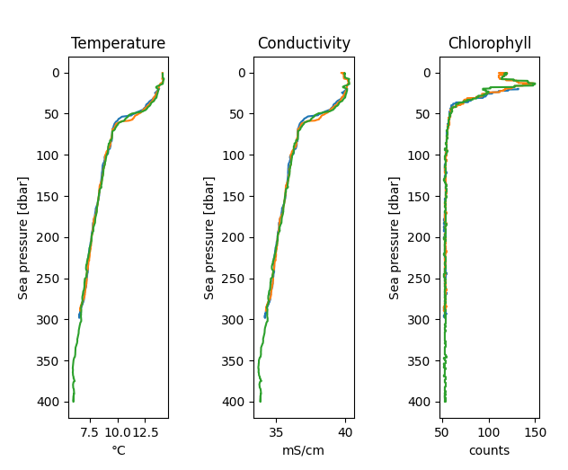
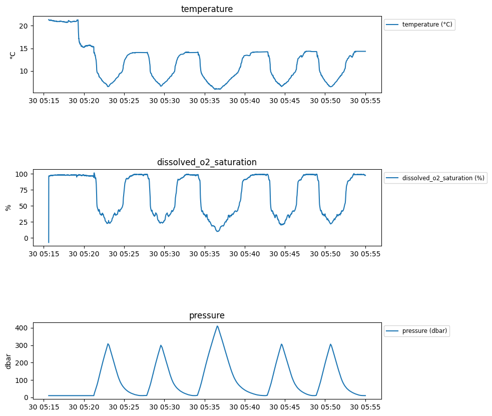
In the case where no profile is available, data can still be plotted as a time series with RSKplotdata().
RSKplotdata(rsk);
Customizing plots
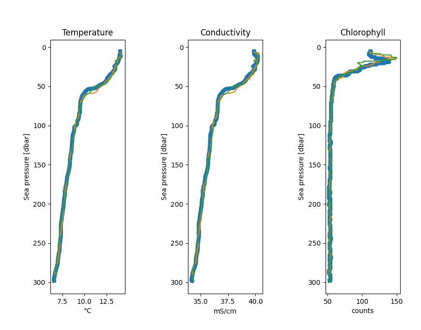
The plotting functions generate standard MATLAB figures. You can modify them using standard MATLAB graphics commands after the function call. For example, to change the line width of the first profile:
RSKplotprofiles(rsk, 'channel', {'Temperature'}, 'direction', 'up');
ax = gca;
ax.Children(1).LineWidth = 3;
Multi-schedule support
With Gen3.5 and Gen4 loggers, RBR instruments can have sensors working at different sampling rates at the same
time. Their data are stored in different schedules with the introduction of the 3.0.0 schema RSK. RSKtools
reads all schedules automatically with RSKreaddata() and stores them in a cell array
rsk.dataArrays. rsk.dataArrays{1} holds schedule 1 data, rsk.dataArrays{2} holds
schedule 2 data, and so on. rsk.data is a convenience alias for rsk.dataArrays{1}.
Each schedule has a label (e.g., 's.CTD', 's.ODO') that identifies its sensor group.
Use rsk.schedules to see available schedules and their labels.
To check how many schedules an RSK file contains:
rsk = RSKopen('sample_multi_schedule.rsk');
disp(rsk.scheduleNumber);
% 2

disp(rsk.schedules);
% scheduleID: 1    label: 's.CTD'
% scheduleID: 2    label: 's.ODO'
How schedule / schedules is used across functions
RSKtools functions accept a schedule or schedules parameter to control which schedule(s)
to operate on. The parameter accepts schedule labels (strings), not integer IDs.
Derive functions (e.g.,
RSKderivesalinity(),RSKderiveseapressure()) accept'schedules'(plural). Default is'all', meaning they derive for all schedules. A single label or cell array of labels can be passed to target specific schedules.Post-processing functions (e.g.,
RSKsmooth(),RSKbinaverage(),RSKremoveloops()) accept'schedule'(singular). Default is'default', which auto-detects the best schedule (the one with the most Conductivity data, then Temperature, then schedule 1).Plot functions (e.g.,
RSKplotdata()) accept'schedules'(plural). Default is'all'.Export functions (e.g.,
RSK2CSV()) accept'schedules'(plural). Default is'all'(one CSV per schedule).
Working with a multi-schedule RSK file
Read data as usual — all schedules are read automatically:
rsk = RSKreaddata(rsk);

% Schedule 1 data
disp(size(rsk.dataArrays{1}.values));

% Schedule 2 data
disp(size(rsk.dataArrays{2}.values));
Derive functions default to all schedules:
rsk = RSKderiveseapressure(rsk);

% Or derive for a specific schedule by label
rsk = RSKderivesalinity(rsk, 'schedules', 's.CTD');
Post-processing functions operate on one schedule at a time:
rsk = RSKreadprofiles(rsk);
rsk = RSKsmooth(rsk, 'channel', 'Temperature', 'windowLength', 5, 'schedule', 's.CTD');
rsk = RSKbinaverage(rsk, 'binBy', 'Sea Pressure', 'binSize', 0.25, ...
                    'direction', 'down', 'schedule', 's.CTD');
Plot data from a specific schedule or all schedules:
% Plot all schedules
RSKplotdata(rsk);

% Plot only the CTD schedule
RSKplotdata(rsk, 'schedules', 's.CTD');
Export a specific schedule to CSV:
RSK2CSV(rsk, 'channel', {'Temperature'}, 'profile', 1, 'schedules', 's.CTD');
Other resources
In addition to the API documentation, we recommend reading the post-processing guide for an introduction on how to process RBR profiles with RSKtools. The post-processing suite contains, among other things, functions to smooth, align, despike, trim, and bin average the data. It also contains functions to export the data to CSV files.