Getting started
Overview
pyRSKtools is RBR’s open source Python toolbox for reading, post-processing, visualising, and exporting RBR logger data. Users may plot data as a time series or as depth profiles using tailored plotting utilities. Time-depth heat maps can be plotted easily to visualise transects or moored profiler data. A full suite of data post-processing functionality, such as methods to match sensor time constants and bin average, are available to enhance data quality. A “sample.rsk” file is available for testing purposes.
Basic usage
The first step is to connect to an RSK file by instantiating an RSK class object. The RSK.open() method
reads various metadata tables from the RSK file which contain information about the instrument channels, sampling configuration,
and profile events. It does not read the instrument data, please refer to the sections below to learn how to read data.
There are two approaches to instantiating and opening an RSK file, as shown below:
Manual approach:
from pyrsktools import RSK

# Instantiate an RSK class object, passing the path to an RSK file
rsk = RSK("/path/to/data.rsk")
# Open the RSK file. Metadata is read here
rsk.open()
# Read, process, view, or export data here
# ...
# Close the RSK file
rsk.close()
Context manager approach:
from pyrsktools import RSK

with RSK("/path/to/data.rsk") as rsk:
    # Read, process, view, or export data here
The second approach uses Python with statement context manager provided by the RSK class to automatically
open the file (at the beginning of the context) and close it (at the end of the context). Except for the syntax,
the context manager approach is functionally the same as the manual approach. For the rest of this document, we
assume an RSK class has been instantiated and assigned to the variable rsk.
An instantiated RSK class may be printed at any time. Printing will provide useful information
about what attributes have been populated so far (including the number of elements in the case of a list/array type attributes).
An example of what printing may look like is provided below:
print(rsk)
RSK
    Internal state attributes:
        .filename is populated
        .logs is populated with 1 elements
        .version is populated
    Informational attributes:
        .appSettings is populated with 1 elements
        .calibrations is populated with 9 elements
        .channels is populated with 5 elements
        .dbInfo is populated
        .deployment is populated
        .epoch is populated
        .instrument is populated
        .instrumentChannels is populated with 9 elements
        .instrumentSensors is populated with 1 elements
        .parameterKeys is populated with 25 elements
        .parameters is populated with 1 elements
        .power is populated with 1 elements
        .ranging is populated with 5 elements
        .regions is populated with 45 elements
        .schedule is populated
        .scheduleInfo is populated
    Computational attributes:
        .data is unpopulated
        .processedData is unpopulated
To learn the differences between internal state, informational, and computational attributes, please refer to the API overview page.
Retrieve metadata from the RSK
Most of the metadata can be shown using print(rsk.metadata_of_interest) once the rsk is opened. For example, to display the instrument channels:
print(rsk.instrumentChannels)
For a list of metadata and information that is stored and can be retrieved in the RSK object, please see RSK.
Reading data from an RSK file
To read data from the instrument, use the RSK.readdata() method. This method will read the full dataset
by default. Because RSK files can store a large amount of data, it may be preferable to read a subset of the
data, specified using start and end times in NumPy datetime64 format. For example:
import numpy as np


t1 = np.datetime64("2022-05-03")
t2 = np.datetime64("2022-05-04")
rsk.readdata(t1, t2)
print(len(rsk.data))
# 77
print(rsk.channelNames)
# ('conductivity', 'temperature', 'pressure')
print(rsk.data["timestamp"])
# ['2020-10-02T18:00:00.000' ...  '2020-10-02T18:10:00.000'  ...]
print(rsk.data["temperature"])
# [15.49902344 15.76919556 12.08074951 ...  8.67211914  ...]
Note that the computational attribute RSK.data is a NumPy array object with column
labels (see NumPy dtype objects) specified by the channel metadata read by
RSK.open(). Refer to the API overview page for more information.
The channel names for each column in RSK.data are contained in
RSK.channelNames (excluding the “timestamp” column). Further, if
you would like to view additional information about channels (such as their units),
you may look into the RSK.channels list or, more conveniently, print them
by running:
rsk.printchannels()

# Model:           RBRconcerto³
# Serial ID:       204571
# Sampling period: 10.0 seconds
# Channels:        index                 name                  unit
#                  _____     ____________________________    ________
#                  0         conductivity                    mS/cm
#                  1         temperature                     °C
#                  2         pressure                        dbar
To plot the data as a time series, use RSK.plotdata().
Working with profile regions
RSK.readdata() reads the instrument data into a single time series as opposed to a series of profile regions.
When Ruskin downloads data from a logger with a pressure channel, it will detect, timestamp, and record profile
upcast and downcast “events” automatically. Users may wish to interact with their data as a series of profiles instead of a
time series.
The RSK.getprofilesindices() method reads CTD data and returns a list of profile/cast indices.
In other words, each element in the returned list is a list itself which may be used to index into RSK.data (or RSK.dataArrays["s.CTD"] for a specific schedule)
to get all the data points for that respective profile/cast. For example, to read the upcast and downcast of the first
3 profiles (profiles start at index 0) from the RSK file, run:
rsk.readdata()
profiles = rsk.getprofilesindices(range(0, 3), direction="both")
for profileIndices in profiles:
    print(rsk.data[profileIndices])
After reading the profiles, they may be plotted with RSK.plotprofiles().
Note: If profiles have not been detected by the logger or Ruskin, or if the profile timestamps do not
correctly parse the data into profiles, the method RSK.computeprofiles() can be used.
The pressureThreshold argument, which determines the pressure reversal required to
trigger a new profile, and the conductivityThreshold argument, which determines if the logger
is out of the water, can be adjusted to improve profile detection when the profiles were very shallow, or
if the water was very fresh.
pyRSKtools includes a convenient plotting option to overlay the pressure data with information about the
profile events. See RSK.plotdata() for more details.
Deriving new channels from measured channels
In this particular example, practical salinity can be derived from conductivity, temperature, and
pressure because the file comes from a CTD-type instrument. RSK.derivesalinity() is a wrapper for the
TEOS-10 GSW function gsw_SP_from_C, and adds a new channel called "salinity" as a column
in RSK.dataArrays. The official Python implementation of the TEOS-10 GSW toolbox is freely available
and can be found here.
Salinity is a function of sea pressure, and sea pressure must be derived from the measured total pressure before computing salinity. In the following example, the default value of atmospheric pressure at sea level, 10.1325 dbar, is used:
rsk.deriveseapressure()
rsk.derivesalinity()
A handful of other EOS-80 derived variables are supported, such as potential temperature and density. pyRSKtools also has wrapper methods for a few common TEOS-10 variables such as absolute salinity.
Plotting
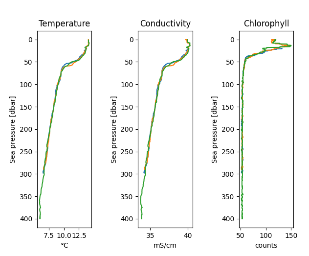
pyRSKtools contains a number of convenient plotting utilities. If the data can be organised as profiles, then it
can be easily plotted with RSK.plotprofiles(). For example, to plot the upcasts of temperature, salinity,
and chlorophyll, run:
import matplotlib.pyplot as plt

fig, axes = rsk.plotprofiles(
    channels=["temperature", "salinity", "chlorophyll"],
    direction="up",
)

plt.show()
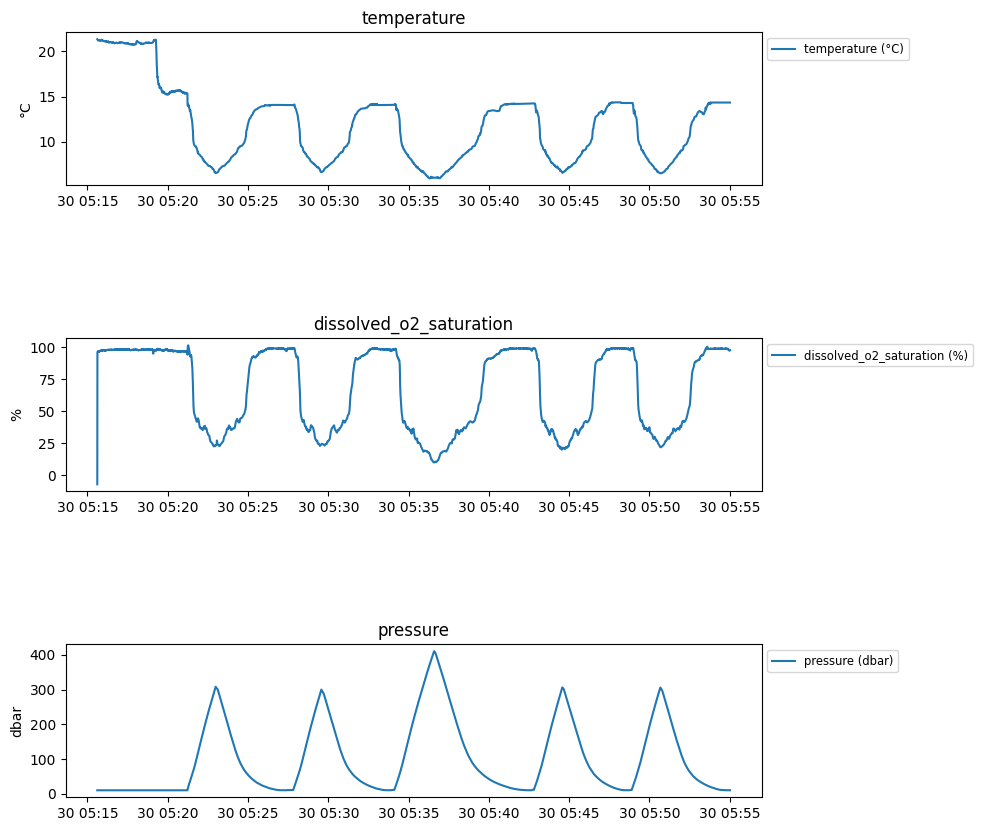
In the case where no profile is available, data can be still plotted as a time series with RSK.plotdata().
For example, to plot temperature, O2 saturation, and pressure as time series, run:
import matplotlib.pyplot as plt

fig, axes = rsk.plotdata(
    channels=["temperature", "dissolved_o2_saturation", "pressure"],
)

plt.show()
Customizing plots
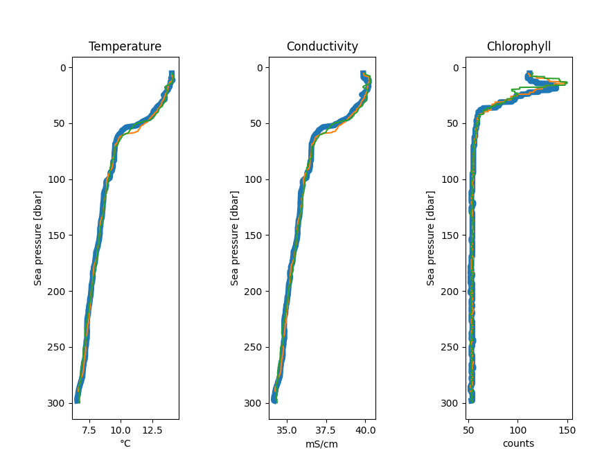
The plotting methods return matplotlib handles to give access to the figure and a list of axes objects (one for each subplot). With such access, you may edit certain properties before showing your plots.
For example, to increase the line width of the first profile in all subplots (before calling plt.show()) of the above example, run:
for ax in axes:
    plt.setp(ax.get_lines()[0], linewidth=6)
Multi-schedule Support
With Gen3.5 and Gen4 loggers, RBR instruments can have sensors working at different sampling rates at the same time. Their data are stored in
different schedules with the introduction of 3.0.0 schema RSK. With a 3.0.0+ schema RSK file containing multiple schedules, RSKtools reads all
data with RSK.readdata() automatically and stores them in RSK.dataArrays, a list where each element holds data for one schedule.
RSK.data is an alias for RSK.dataArrays[0]. You can also retrieve a schedule-specific dataset directly by label, for example
RSK.dataArrays["s.CTD"].
Schedule labels
Each schedule has a label (e.g., "s.CTD", "s.ODO"). These labels are how you tell pyRSKtools which schedule to work with.
You can also retrieve the corresponding metadata directly with rsk.schedules["s.CTD"] and
rsk.scheduleInfos["s.CTD"]. Always check the available labels before processing:
for i, sched in enumerate(rsk.schedules, start=1):
    info = rsk.scheduleInfos[sched.label]
    print(
        f"Schedule {i}: label='{sched.label}', mode={sched.mode}, "
        f"sampling period={info.samplingperiod()}s"
    )
How schedules are used across functions
Derive functions (e.g.,
RSK.derivesalinity()) acceptschedules(plural) and default to"all". They derive the wanted channel for every schedule, using the most recent available measurement from any schedule for each timestamp.Post-processing functions (e.g.,
RSK.despike()) acceptschedule(singular) and default to"default", which auto-detects the schedule with the most non-NaN conductivity data, then temperature, and falls back to schedule 1 if neither channel is available. Post-processing parameters are often schedule-specific, so these functions operate on one schedule at a time.RSK.computeprofiles()is another exception: itsschedule="default"picks the schedule containing the most non-NaN pressure data, then sea pressure.RSK.calculateCTlag()is the main exception: itsschedule="default"picks the schedule containing both conductivity and temperature with the most non-NaN data in both channels.Plot functions (e.g.,
RSK.plotdata()) acceptschedules(plural) and default to"all". A list matching the number of channels can be passed for per-channel schedule control.RSK.images()is another exception: it operates on one schedule at a time and defaults toschedule="default", using the same single-schedule auto-detection as other schedule-specific functions.
Working with an RSK file with multiple schedules
To work with an RSK file with multiple schedules, read the data as usual:
rsk.readdata(t1, t2)
To inspect schedules and their data:
print(rsk.scheduleNumber)  # how many schedules

print(rsk.schedule)        # first schedule (alias for schedules[0])
print(rsk.scheduleInfo)    # first schedule info
print(rsk.data[:4])        # first 4 data points from schedule 1

print(rsk.schedules["s.ODO"])         # schedule labelled s.ODO
print(rsk.scheduleInfos["s.ODO"])     # info for schedule labelled s.ODO
print(rsk.dataArrays["s.ODO"][:4])    # first 4 data points from the s.ODO schedule
When an RSK has multiple schedules, it can still have recorded regions of profiles. To manually compute profiles, specify the schedule label:
rsk.computeprofiles(schedule="s.CTD") # use CTD data to compute profiles
To plot data from multiple schedules:
# Plot all channels from all schedules
rsk.plotdata()

# Plot specific channels from a single schedule
rsk.plotdata(channels=["temperature", "conductivity"], schedules="s.CTD")

# Mix-and-match: per-channel schedule control
rsk.plotdata(
    channels=["temperature", "dissolved_o2_concentration"],
    schedules=["s.CTD", "s.ODO"],
)
For schedule-specific plots like a T-S diagram:
rsk.plotTS(schedules="s.CTD")
Derive functions default to all schedules. Even if a schedule lacks temperature measurements, salinity can still be derived using the last available measurement from other schedules:
rsk.deriveseapressure()  # derives for all schedules by default

# Or derive for specific schedules only
rsk.derivedepth(schedules="s.CTD")
rsk.derivevelocity(schedules="s.CTD")
Post-processing functions operate on one schedule at a time. Specify the schedule label explicitly:
rsk.binaverage(direction="down", binSize=20.0, boundary=0.5, schedule="s.CTD")
rsk.binaverage(direction="down", binSize=50.0, boundary=0.5, schedule="s.ODO")
To export a multi-schedule RSK to CSV:
rsk.RSK2CSV(outputDir="./output")  # exports all schedules, one CSV per schedule
rsk.RSK2CSV(outputDir="./output", schedules="s.CTD")  # export only CTD schedule
To export as a full schema RSK file (EPdesktop RSK does not support multiple schedules):
rsk.RSK2RSKFULL(inputPath="sample_multi_schedule.rsk", outputDir="./output", suffix="processed")
Other resources
In addition to the API documentation, we recommend reading the post-processing guide for an introduction on how to process RBR profiles with pyRSKtools. The post-processing suite contains, among other things, methods to smooth, align, de-spike, trim, and bin average the data. It also contains methods to export the data to CSV files.